Introduction¶

The aim of this practical session is to get yourself acquainted with the ill-balanced nature of NLP classification tasks and to get some exposure to the scikit-learn and spaCy packages.

A great example of a highly-biased task is spam classification. The goal of the task is to classify whether a given piece of text (e.g., email, sms message) is spam or not. Since there are only 2 classes (spam or not), we call such tasks binary classification.

In reality, the amount of examples we have of non-spam emails is much larger than the ones that are spam. Therefore, we need proper evaluation techniques to deal with such a class imbalance.

Fun fact: if a piece of text is not spam, it's popularly called ham!

Content Warning: this exercise's data will contain explicit words.¶

Setting up your environment¶

While you can downlaod the following packages with pip to your computer directly, we recommend (but not require) you to use a virtual environment to not mess up the package versions for different project. If you'd like to, here is a quick tutorial on virtual environments that you can checkout with an EPFL email.

First make sure you have (a virtual environment (e.g., venv, virtualenv, conda), and that the environment has) a Python version >= 3.6, per spaCy package requirements. If you are using the a Jupyter Notebook, make sure the interpreter points to the correct python executable.

Then install the following packages:

pip install -U ipykernel
pip install -U pip setuptools wheel
pip install -U pandas
pip install -U matplotlib
pip install -U scikit-learn
pip install -U seaborn
pip install -U spacy
pip install -U classy-classification

python -m spacy download en_core_web_sm

Next, import the necessary packages:

Note: if this part of the code hangs, simply restart your kernel and rerun, sometimes importing packages multiple times can create a problem

In [ ]:

# Importing necessary packages:
import spacy
import classy_classification
import pandas as pd
import numpy as np
import os
import random
import matplotlib.pyplot as plt
import seaborn as sns
from sklearn.metrics import accuracy_score, precision_score, recall_score, f1_score, confusion_matrix, precision_recall_curve
from sklearn.model_selection import train_test_split, KFold
from sklearn import metrics

# Setting the seed:
seed = 42
os.environ['PYTHONHASHSEED']=str(seed)
random.seed(seed)
np.random.seed(seed)

# Setting print options for readability:
pd.set_option('display.max_columns', None)
pd.set_option('display.expand_frame_repr', False)
pd.set_option('max_colwidth', None)

Now you are ready to start the exercises!

1) Brief Data Analysis & Processing¶

To evaluate the spam task, we will use an annotated English sms corpus from Kaggle. You can download the data here. Run the following 2 blocks of code to see what the data looks like:

In [ ]:

df = pd.read_csv("spam.csv", header=0, names=['label','sms'], usecols=[0,1])
df.head()

As you can see there are 2 types of classes: "ham" & "spam". Let's take a look at their distribution:

In [ ]:

print("Label counts are:")
print(df.label.value_counts())

print("______________________")
print("Label percentages are:")
print(df.label.value_counts(normalize=True))

Q: How is this dataset's label distribution imbalanced? Which datapoints are more common?

A: TODO - your answer here!

Let's do some minor data processing. We map the labels {"ham" $\implies$ 0} and {"spam" $\implies$ 1} as our goal is to identify spam messages.

In [ ]:

df['label'] = df['label'].replace(to_replace={'ham': 0, 'spam': 1})
df.head()

Then, to make sure that we don't overfit our models to the data, we split the data into train and test sets. We use the very convenient train_test_split function from scikit-learn. The test_size parameter allows us to choose what percentage of the data should be in the test set. $x$ is the sms message, while $y$ is the corresponding label to the sms.

Remember, when you are prototyping a model, never use the test data. The goal of the test data is to simulate an independently sampled dataset, that cannot be seen during training and model designing. Extracted statistics should come from the training set only.

In [ ]:

x_train, x_test, y_train, y_test = train_test_split(df['sms'].values, df['label'].values, test_size=0.2, random_state=seed)

print("Spam amount in train set: {} out of {} datapoints".format((y_train == 1).sum(), len(y_train)))
print("Spam percentage in train set: {}%".format(round((y_train == 1).sum() / float(len(y_train)) * 100, 4)))

print("Size of train set is: ", len(y_train))
print("Size of test set is: ", len(y_test))

2) Simple & Random Classifiers¶

Our first task is to evaluate simple classifiers to see how well they do on the spam classification task. Note that while there is a text input, none of these classifiers actually care about the content of the string. Remember that a prior in probability is one's belief about a quantity given some past evidence.

rand_binom_uniform_classifier: The first model uniformly randomly classifies the label for a given piece of text, meaning the prior is $p=0.5$.
rand_binom_biased_classifier: The second model binomally samples a label, you should chose which prior $p$ you think makes the most sense!
always_false_classifier: The third model returns always false, basically assuming that no text can ever be spam.

Don't forget to change the value prior_p $=0.5$! Chose the value informatively! Think which statistics can help you with this.

In [ ]:

##############################
# TODO: write a prior you think that makes the most sense in the next line for the rand_binom_biased_classifier:
prior_p = 0.5 # <-------- CHANGE THIS VALUE!
##############################

def rand_binom_uniform_classifier(text):
    """
    Unfiormly randomly picks a binary label.
    Returns ints 0 or 1.
    """
    return np.random.binomial(n=1, p=0.5)

def rand_binom_biased_classifier(text):
    """
    Randomly picks a binary label according to a prior_p.
    Returns ints 0 or 1.
    """
    return np.random.binomial(n=1, p=prior_p)

def always_false_classifier(text):
    """
    Always returns int 0.
    """
    return 0

def predict(model, dataset):
    """
    Applies model prediction on every sentence.
    """
    return [model(text) for text in dataset]

Now we are going to use the accuracy_score metric provided by scikit-learn:

In [ ]:

rand_binom_uniform_preds = predict(rand_binom_uniform_classifier, x_test)
rand_binom_biased_preds = predict(rand_binom_biased_classifier, x_test)
always_false_preds = predict(always_false_classifier, x_test)

for model_name, model in [
        ("Rand Uniform", rand_binom_uniform_classifier), 
        ("Rand Binom p={}".format(prior_p), rand_binom_biased_classifier), 
        ("Always False", always_false_classifier)]:
    test_preds = predict(model, x_test)
    test_accuracy = accuracy_score(y_test, test_preds) # NOTE: here we pass the gold labels and the predicted labels to calculate how well our model is doing
    print("Model: {} || Accuracy: {}%".format(model_name, round(test_accuracy * 100, 4)))

Wow! Looks like the "Always False" classifier is amazing at this task, even better than randomly choosing. Over 85% sounds like a pretty good result. Can we call it quits, and go home now? Not so fast... Answer the following questions.

Q: Which prior did you choose and why do you think it fits the problem? If you chose your prior informatively, the Rand Binom classifier should be better than the Rand Uniform classifier. Why is the biased random classifier doing better than the uniform one?

A: TODO - your answer here!

Q: How would using testing data to design the model be "bad practice"? Give an example.

A: TODO - your answer here!

Q: Why is the accuracy score not the correct metric to use in this task? Which classifier is a good example of this? What other metrics can be used and why would they be a better fit for this task?

A: TODO - your answer here!

2.2) Precision, Recall, F1-score & Friends¶

Now that you have convinced yourself that accuracy is not the sole metric we should be using. For the other possible scores we let you explore the following metrics conveniently provided by scikit-learn:

precision_score
recall_score
f1_score
confusion_matrix - while this is not a metric, it allows to visualize the true positives, true negatives, false positives, and false negatives (TP, TN, FP, FN)

Note that some of these function also has a zero_division parameter as the denominator of these metrics can be validly 0. In that case the default is to also output 0, but a warning may be raised. Feel free to ignore the warning.

TIP: Can you not remember what precision and recall is? Remember it with the start of the word:

Precision: PREcision is TP divided by PREdicted positive:

$ \frac{TP}{TP+FP}$
Recall: REcAll is TP divided by REAl positive: TP/(TP+FN)

$ \frac{TP}{TP+FN}$

source: stats.stackexchange

In [ ]:

for model_name, model in [
        ("Rand Uniform", rand_binom_uniform_classifier), 
        ("Rand Binom p={}".format(prior_p), rand_binom_biased_classifier), 
        ("Always False", always_false_classifier)]:
    
    test_preds = predict(model, x_test)
    
    test_accuracy = accuracy_score(y_test, test_preds)
    test_precision = precision_score(y_test, test_preds)
    test_recall = recall_score(y_test, test_preds)
    test_f1 = f1_score(y_test, test_preds)
    cf_train_matrix = confusion_matrix(y_test, test_preds)

    # print("________________________________________________________________")
    print("Model: {}".format(model_name))
    print("\t|| Accuracy: {}% ".format(test_accuracy))
    print("\t|| Precision: {}% ".format(test_precision))
    print("\t|| Recall: {}% ".format(test_recall))
    print("\t|| F1: {}% ".format(test_f1))

    plt.figure(figsize=(2.5,2))
    sns.heatmap(cf_train_matrix, annot=True, fmt='d')
    plt.xlabel("Predicted Labels")
    plt.ylabel("Real Labels")
    plt.show()

Q: What do precision, recall, or the confusion metrics tell us about the "Always False" model? Why don't we see this phenomenon with the random classifiers?

A: TODO - your answer here!

Q: What would be a more ideal confusion matrix result?

A: TODO - your answer here!

3) Big IF Keyword-Matching Classifier¶

So far, our models haven't taken into account the actual text. In this next task we build the most simple AI algorithm: a big IF statement that classifies the text as spam if a "spam word" is being used. To do so we first have to break the sentence down into words. Assuming we only have English sentences, we can separate them by space or punctuation. This action of breaking a sentence into tokens is called tokenization. For now instead of using the spaCy implementation, let's create our own simple tokenizer that turns a sentence into a list of tokens by splitting on empty spaces.

Consider the sentence: "I am not a spam message, don't confuse me with it!" There are many ways we could break it into tokens:

With just space:
- ['I', 'am', 'not', 'a', 'spam', 'message,', "don't", 'confuse', 'me', 'with', 'it!']
Separate punctuation as well:
- ['I', 'am', 'not', 'a', 'spam', 'message', ',', "don't", 'confuse', 'me', 'with', 'it', '!']
Separating on apostrophe:
- ['I', 'am', 'not', 'a', 'spam', 'message', ',', 'do', "n't", 'confuse', 'me', 'with', 'it', '!']

You could even tokenize sentence into subword elements. For example, it won't be very interesting, but you could even break it into characters!:

['I', 'a', 'm', 'n', 'o', 't', 'a', 's', 'p', 'a', 'm', 'm', 'e', 's', 's', 'a', 'g', 'e', ',', 'd', 'o', 'n', "'", 't', 'c', 'o', 'n', 'f', 'u', 's', 'e', 'm', 'e', 'w', 'i', 't', 'h', 'i', 't', '!']

In [ ]:

def simple_tokenizer(text):
    return text.split(" ")

def custom_tokenizer(text):
    pass # TODO: OPTIONAL, have fun! Implement your own tokenizer that's more elegant than the above one

print(simple_tokenizer("I am not a spam message, don't confuse me with it!"))
print(custom_tokenizer("I am not a spam message, don't confuse me with it!"))

Let's take a look at what our tokenizer does on our dataset:

In [ ]:

x_tokenized_test = [simple_tokenizer(sentence) for sentence in x_test]
for i in [5, 6, 2]:
    print("__________________________________________________________________")
    print("Label: ", y_test[i])
    print("Sentence: ", x_test[i])
    print("Tokenized version: ", x_tokenized_test[i])

In [ ]:

# TODO: Change or fill more with words you think indicate a spam message!
spam_words = ["money", "drugs", "winner"]

Now let's implement our keyword matching algorithm:

In [ ]:

def big_if_classifier(text):
    tokenized_text = simple_tokenizer(text)
    for token in tokenized_text:
        if token in spam_words:
            return 1
    return 0

Next, we evaluate the big if classifier:

In [ ]:

for model_name, model in [("Big If", big_if_classifier)]:
    
    test_preds = predict(model, x_test)
    test_accuracy = accuracy_score(y_test, test_preds)
    test_precision = precision_score(y_test, test_preds)
    test_recall = recall_score(y_test, test_preds)
    test_f1 = f1_score(y_test, test_preds)

    print("Model: {}".format(model_name))
    print("\t|| Accuracy: {}% ".format(test_accuracy))
    print("\t|| Precision: {}% ".format(test_precision))
    print("\t|| Recall: {}% ".format(test_recall))
    print("\t|| F1: {}% ".format(test_f1))

    cf_train_matrix = confusion_matrix(y_test, test_preds)
    plt.figure(figsize=(2.5,2))
    sns.heatmap(cf_train_matrix, annot=True, fmt='d')
    plt.xlabel("Predicted Labels")
    plt.ylabel("Real Labels")
    plt.show()

Q: What are some of the shortcomings of this big-if classifier? How could you mitigate such problems?

A: TODO - your answer here!

Q: What are some other linguistic features you think that could help classify spam messages without having as many false-negatives? To check what type of linguistic features you can extract with spacy, take a look at this page.

A: TODO - your answer here!

4) SpaCy Classifier¶

Loading the following classifier can take from 0.5-7 minutes depending on your internet connection, so start running this code while reading the rest of the notebook (ignore the warnings!):¶

In [ ]:

# NOTE: Ignore the content of this code. Simply run it :)

# -) Reformatting data for spacy text categorizer
#    The few-shotness comes from the fact that we only train with 200 examples from the actual ~4000 training examples we have
train_data_dict = {
    "1": [],
    "0": []
}
for i in range(200): 
    label_str = str(y_train[i])
    train_data_dict[label_str] = train_data_dict[label_str] + [x_train[i]]

# -) Load the spacy text categorizer / few-shot learn from the reformatted examples
spacy_classifier = spacy.load("en_core_web_sm") # nlp = spacy.blank("en") 
spacy_classifier.add_pipe(
    "text_categorizer", 
    config={
        "data": train_data_dict, 
        "model": "sentence-transformers/paraphrase-multilingual-MiniLM-L12-v2",
        "device": "cpu"
    }
)

The following classifier will be a classifier trained with spacy that you will learn later on in the course. For now focus on the evaluation & some cool aspects of this package.

You may have noticed that our tokenization is too simple. "money" could be written right before a comma, and apostrophes might also create duplicate tokens that actually refer to the same word. Spacy provides a tokenizer for different languages that takes care of such edge cases.

And that's not only it! The framework is organized as a pipeline that takes a plain string text and turns it into a featurized Doc. Document here doesn't mean multiple sentences. You can think of Doc as an augmentation of the plain text into meaningful linguistic features that can be better signals for classification tasks. Here is a possible set of components to make up the spacy nlp pipeline:

NLP Pipeline

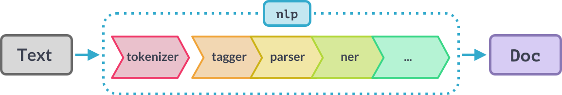
Notice that the tokenizer is separate. This is because for a given language, spaCy has only one tokenizer. As said on the website:

[...] while all other pipeline components take a Doc and return it, the tokenizer takes a string of text and turns it into a Doc

So let's create an English pipeline with only the tokenizer by disabling the rest of the components.

First, we need to load the language specific nlp pipeline with spacy.load(). Then there are 2 ways to pass text into spacy.

You can process an individual string with:
```
 nlp(text)
```
You can process a stream of multiple strings with:
```
 nlp.pipe(texts)
```

In [ ]:

sample_texts = [
    "This message is not a spam, believe me!!",
    "I AM DEFINETLY A SPAM, give me 2000$, I need money, please help!",
    "I am not a spam message, don't confuse me with it!"
]

# 1) Load the language specific NLP pipeline
nlp = spacy.load("en_core_web_sm")
print("The default English nlp pipe components are: {}. We disable them in the pipe call.\n".format(nlp.pipe_names))

# 2) Process multiple texts with the nlp.pipe function
for doc in nlp.pipe(sample_texts, disable=['tok2vec', 'tagger', 'parser', 'attribute_ruler', 'lemmatizer', 'ner']):
    print([token.text for token in doc])

In [ ]:

print(spacy_classifier("I am looking for kitchen appliances.")._.cats)

In [ ]:

print(spacy_classifier("For only 1000$, you can also be a winner!")._.cats)

Wow! The predicted probabilities for each label seem quite reasonable. Now let's test this on the whole test dataset:

In [ ]:

def predict_spacy(model, dataset):
    preds = []
    for doc in model.pipe(dataset):
        res_dict = doc._.cats
        pred = int(max(res_dict, key=res_dict.get)) # NOTE: this is one way to argmax in python
        preds.append(pred)
    return preds

Evaluating with the spacy classifier takes longer than our models, so note that the following may take around a minute:

In [ ]:

for model_name, model in [("Spacy", spacy_classifier)]:
    
    test_preds = predict_spacy(model, x_test)
    
    test_accuracy = accuracy_score(y_test, test_preds)
    test_precision = precision_score(y_test, test_preds)
    test_recall = recall_score(y_test, test_preds)
    test_f1 = f1_score(y_test, test_preds)
    cf_train_matrix = confusion_matrix(y_test, test_preds)

    print("________________________________________________________________")
    print("Model: {}".format(model_name))
    print("\t|| Accuracy: {}% ".format(test_accuracy))
    print("\t|| Precision: {}% ".format(test_precision))
    print("\t|| Recall: {}% ".format(test_recall))
    print("\t|| F1: {}% ".format(test_f1))

    plt.figure(figsize=(2.5,2))
    sns.heatmap(cf_train_matrix, annot=True, fmt='d')
    plt.xlabel("Predicted Labels")
    plt.ylabel("Real Labels")
    plt.show()

Q: What can you notice about the precision/recall/F1/confusion matrix results? What is particularly improved compared to the "Big-If" classifier?

A: TODO - your answer here!

5) Statistical Significance & Comparing all Models¶

Now that we have many models under our belt, let's compare the statistical significance of the 4 classifiers:

Rand Binom
Always False
Big If
Spacy

As you learned it lecture, one way to measure stastical significance is by doing a k-cross validation. Once again, scikit-learn has a convenient KFold class that splits a given dataset input and output into k folds. Here we will use k $=5$ which gives us a ratio of 0.2 validation set. We hold out the test set, and do this procedure only on the train set. Note that the following may take 10 minutes to run as the spacy model gets retrained with 200 examples every new k-fold.

In [ ]:

k = 5 # NOTE: You can change the value of k via the argument here!
k_fold = KFold(k)
kfold_iteration = enumerate(k_fold.split(x_train, y_train))

metrics = {
    "Rand Uniform": {
        'acc': [],
        'pre': [],
        'rec': [],
    },
    "Rand Binom p={}".format(prior_p): {
        'acc': [],
        'pre': [],
        'rec': [],
    },
    "Always False": {
        'acc': [],
        'pre': [],
        'rec': [],
    },
    "Big If": {
        'acc': [],
        'pre': [],
        'rec': [],
    },
    "Spacy": {
        'acc': [],
        'pre': [],
        'rec': [],
    },
}

for k, (train_idx, val_idx) in kfold_iteration:
    print("K-cross validation iteration {}".format(k))
    x_tr, x_val = x_train[train_idx], x_train[val_idx]
    y_tr, y_val = y_train[train_idx], y_train[val_idx]

    for model_name, model in [
        ("Rand Uniform", rand_binom_uniform_classifier), 
        ("Rand Binom p={}".format(prior_p), rand_binom_biased_classifier), 
        ("Always False", always_false_classifier),
        ("Big If", big_if_classifier)]:

        val_preds = predict(model, x_val)
        metrics[model_name]['acc'].append(accuracy_score(y_val, val_preds))
        metrics[model_name]['pre'].append(precision_score(y_val, val_preds))
        metrics[model_name]['rec'].append(recall_score(y_val, val_preds))

    for model_name, model in [("Spacy", nlp)]:
        train_data_dict = {
            "1": [],
            "0": []
        }
        for i in range(200): # NOTE: you can increase the training size by making this number larger
            label_str = str(y_tr[i])
            train_data_dict[label_str] = train_data_dict[label_str] + [x_tr[i]]

        nlp = spacy.load("en_core_web_sm") # nlp = spacy.blank("en") 
        nlp.add_pipe(
            "text_categorizer", 
            config={
                "data": train_data_dict, 
                "model": "sentence-transformers/paraphrase-multilingual-MiniLM-L12-v2",
                "device": "cpu"
            }
        )    
        val_preds = predict_spacy(nlp, x_val)
        metrics[model_name]['acc'].append(accuracy_score(y_val, val_preds))
        metrics[model_name]['pre'].append(precision_score(y_val, val_preds))
        metrics[model_name]['rec'].append(recall_score(y_val, val_preds))

In [ ]:

acc_means = []
acc_stds = []
pre_means = []
pre_stds = []
rec_means = []
rec_stds = []

model_names = list(metrics.keys())
for model in model_names:
    acc_means.append(np.mean(metrics[model]['acc']))
    acc_stds.append(np.std(metrics[model]['acc']))
    #
    pre_means.append(np.mean(metrics[model]['pre']))
    pre_stds.append(np.std(metrics[model]['pre']))
    #
    rec_means.append(np.mean(metrics[model]['rec']))
    rec_stds.append(np.std(metrics[model]['rec']))

x = np.arange(len(model_names))
width = 0.25

fig, ax = plt.subplots()
rects1 = ax.bar(x, acc_means, width,  yerr=acc_stds, label='Accuracy', edgecolor = 'black')
rects1 = ax.bar(x + width , pre_means, width,  yerr=pre_stds, label='Precision', edgecolor = 'black')
rects2 = ax.bar(x + width * 2, rec_means, width,  yerr=rec_stds, label='Recall', edgecolor = 'black')

ax.set_ylabel('Metric value')
ax.set_title('k=5-cross validation metric variance')
ax.set_xticks(x + width, model_names, rotation = 30)
ax.legend()

fig.tight_layout()
plt.show()

Spam Classification Evaluation¶

Introduction¶

Content Warning: this exercise's data will contain explicit words.¶

Setting up your environment¶

1) Brief Data Analysis & Processing¶

2) Simple & Random Classifiers¶

2.1) Accuracy¶

2.2) Precision, Recall, F1-score & Friends¶

3) Big IF Keyword-Matching Classifier¶

4) SpaCy Classifier¶

Loading the following classifier can take from 0.5-7 minutes depending on your internet connection, so start running this code while reading the rest of the notebook (ignore the warnings!):¶

5) Statistical Significance & Comparing all Models¶